TL;DR: Kolmogorov-Arnold Networks replace scalar edge weights with learnable one-dimensional functions, usually splines in the original design, so each connection learns a curve instead of a number.[1] One Poisson PDE experiment reported 100 times lower squared error with 100 times fewer parameters, but the same paper disclosed a typical 10-times training slowdown at equal parameter count.[1] By 2026, accepted work had extended KANs into symbolic neural operators, hardware-aware transformers, multivariate lookup layers, and restricted training theory, but every major success changed or constrained the original spline design.[8][10][12][13]
KANs arrived in April 2024 with the kind of pitch the AI industry cannot resist. Change one foundational assumption, then make decades of neural-network design look unnecessarily rigid. Multi-layer perceptrons, or MLPs, learn scalar weights between neurons and apply fixed nonlinear activations on the neurons. KANs put learnable nonlinear functions on the connections instead.
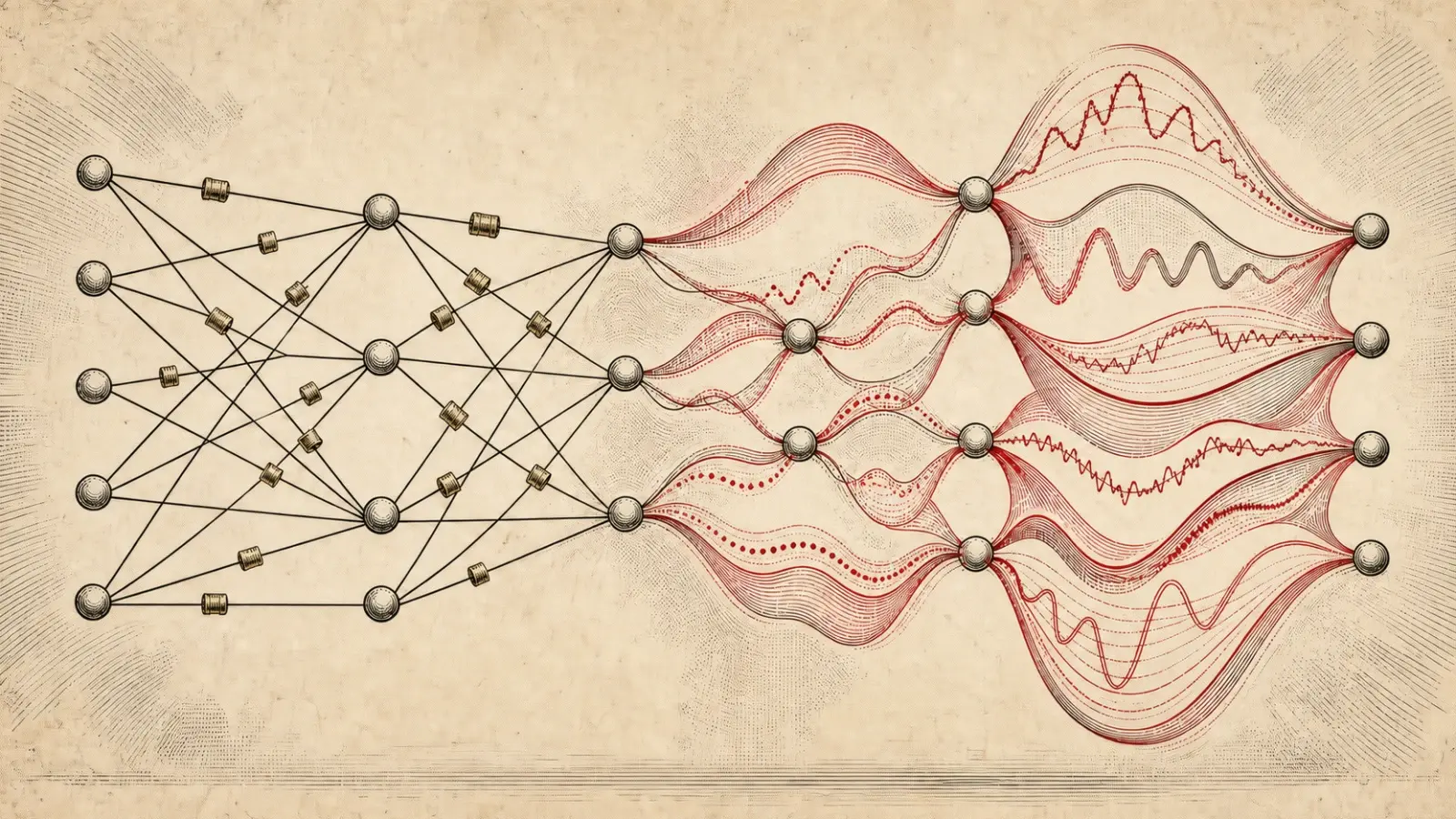
That sounds cosmetic. It is not. A scalar weight can only amplify, suppress, or reverse a signal. A learned function can bend, saturate, oscillate, flatten, or sharpen the signal differently at every input value. The connection stops being a volume knob and becomes a tiny curve-fitting machine.
The real story isn't that KANs killed the MLP. They did not. The real story is that KANs exposed a valuable design axis: a network can learn the shape of a connection, not merely its strength. The research since 2024 has been a two-year stress test of when that extra freedom earns its cost.
Why This Matters Now
The follow-up record is no longer empty. Accepted 2025-2026 work now spans KANO at ICLR, FlashKAT at AAAI, KAN optimization and privacy theory at ICML, lmKAN scaling at ICLR, ReLU convertibility at AISTATS, and a peer-reviewed warning that scientific model discovery can be nonunique.[4][5][8][10][12][13] The real 2026 verdict is not that KANs replaced MLPs. It is that learnable functional connections became a serious research program.
The Architecture: Every Connection Learns A Curve
A conventional MLP layer performs two familiar operations. It multiplies an input vector by a matrix of learned scalar weights, adds biases, then applies a fixed activation such as ReLU, GELU, or tanh at each node.
A KAN layer reorganizes that bargain. For every connection from input coordinate i to output coordinate j, the network learns a univariate function phi[j,i]. Each output coordinate is the sum of those transformed inputs:
x_next[j] = sum_i phi[j,i](x[i])
There is no single shared activation curve sitting on the destination node. Every edge can learn its own curve. In the original PyKAN design, that curve combines a residual base function with a trainable B-spline expansion. The model adjusts multiple coefficients over a grid, allowing one edge to behave differently across different input regions.[1][1]
MLP Versus KAN: Where The Learning Lives
| Feature | MLP | Original KAN |
|---|---|---|
| One connection | One learned scalar | One learned univariate function |
| Nonlinearity | Fixed activation on nodes | Learned activation on edges |
| Typical primitive | Matrix multiply plus GELU | Spline evaluation plus summation |
| Same-width parameter scale | O(N²L) | O(N²L(G+k)) |
| Systems advantage | Dense, optimized hardware path | Flexible local function fitting |
Here is the genius. B-spline basis functions have local support. Adjusting one coefficient changes a limited region of a curve instead of rewriting its entire shape. PyKAN can also extend a trained spline grid from coarse to fine, preserving the learned function while adding local resolution.[1]
The cost appears immediately. One MLP edge stores one number. One original KAN edge stores multiple spline coefficients and scales. For width N, depth L, grid size G, and spline order k, the original paper gives KAN parameter scaling of O(N²L(G+k)), versus O(N²L) for an MLP of comparable width and depth.[1]
KANs are therefore not inherently smaller. They become smaller only if their richer edges let the network use substantially less width or depth for the target problem.
The Mechanics: From Data To An Inspectable Formula
The Kolmogorov-Arnold representation theorem says a continuous multivariate function on a compact domain can be written using sums and compositions of continuous univariate functions. KANs borrow that compositional intuition and make the univariate functions trainable.[1]
The theorem is an existence result, not an optimization guarantee. It does not promise that gradient descent will discover a compact factorization, that B-splines are the best basis, or that the resulting functions will be easy to interpret. Those are engineering and statistical questions.
How A Spline KAN Learns
The training loop turns scalar connections into locally adjustable functions.
Initialize Edge Functions
Each connection starts with a base activation and a low-resolution spline over an input grid.
Transform Each Input
Every scalar input passes through the function on its outgoing edge. A destination node sums the transformed values.
Update Curve Coefficients
Backpropagation changes spline coefficients and scaling parameters to reduce task loss.
Extend The Grid
The model can interpolate a trained curve onto a finer grid, adding local resolution without restarting.
Prune And Symbolize
Weak edges are removed, then useful curves can be matched to candidate symbolic functions and validated.
Suppose a target contains sin(x1) or x2². An MLP can approximate the relationship across many scalar weights and hidden activations. A compact KAN can learn an edge curve that visually resembles the term. A researcher can prune weak edges, inspect the surviving curves, replace a curve with a candidate symbolic function, retrain, and test whether the simpler expression preserves accuracy.[1]
That is a real interpretability advantage, but it is not automatic truth. A plotted spline is still an approximation learned from finite data. Symbolic snapping uses a function library, thresholds, regularization, and sometimes human judgment. Small, sparse KANs can be legible. A million edge functions would be another black box with better diagrams.
A KAN edge is not an explanation. It is a testable hypothesis drawn as a curve.
The Original Evidence: A Spectacular Result With Boundaries
The first paper tested synthetic function fitting, special functions, a Poisson partial differential equation, knot classification, and controlled physics examples. Its most repeated number came from the Poisson setup. A two-layer, width-10 KAN reached a reported 10^-7 squared error, versus 10^-5 for a four-layer, width-100 MLP. The paper described that as 100 times better accuracy and 100 times better parameter efficiency in that experiment.[1]
The Poisson Result That Launched KANs
These figures belong to one controlled PDE experiment, not a universal scaling law.
Reported squared error for a two-layer, width-10 KAN
Reported squared error for a four-layer, width-100 MLP
Reported advantage for the smaller KAN in this experiment
Authors' typical KAN slowdown at equal parameter count
Let's be clear. This was compelling evidence that KANs fit certain low-dimensional, compositional scientific functions unusually well. It was not evidence that a billion-parameter KAN would replace a language model, a vision backbone, or every MLP block inside a transformer.
What's often overlooked is that the authors disclosed the systems weakness themselves. At equal parameter count, their KAN implementation was typically 10 times slower to train than an MLP. They also acknowledged that the analytic PDE solution could favor KANs because the architecture is unusually well suited to symbolic formulas.[1]
The uncomfortable truth is that parameter count was the flattering metric. Each KAN parameter lived inside a more expensive computational path than a scalar in a dense matrix multiplication.
The Follow-Ups: The Idea Survived By Changing Form
KAN 2.0 clarified the most credible destination in August 2024. Instead of pitching a universal layer replacement, it described a two-way scientific workflow. Science-to-KAN injects candidate variables, formulas, and domain constraints. KAN-to-science prunes the graph, exposes modules, and converts useful curves into symbolic conjectures. MultKAN added explicit multiplication nodes, kanpiler compiled formulas into trainable KANs, and a tree converter exposed modular structure.[2]
The paper's most revealing result was not a feature. It was a failure of prior knowledge. In one Neo-Hookean constitutive-law experiment, a prior-informed route ended with a reported loss of 7 × 10^-3 for the P12 term. A randomly initialized route recovered 0.42(F11F21 + F12F22 + F13F23) with a loss of 6 × 10^-9.[2] The authors warned against generalizing from one case, but the lesson was sharp: scientific priors can guide discovery and also trap optimization in a bad basin.
That makes KAN 2.0 an interactive conjecture engine, not an autonomous scientist. Researchers still decide what variables to expose, which edges to prune, which symbolic library to search, and whether a compact expression is physically meaningful.
The 2025 Warning: Predictive Fidelity Does Not Identify One Law
A peer-reviewed 2025 Physical Review Research paper pushed KANs into non-sparse chaotic dynamics, including the Ikeda optical-cavity map. Its models reproduced invariant sets and system statistics, including Lyapunov behavior and distributional measures, without requiring the governing law to be sparse in a small hand-built term library.[4]
The finding came with a deeper warning. Multiple learned models could reproduce the same invariant set and statistics. A KAN can therefore fit the observable dynamics and still fail to identify a unique underlying law. Predictive fidelity does not eliminate epistemic ambiguity.
This is not a weakness unique to KANs. It is a boundary on the entire scientific-discovery pitch. A readable formula can be wrong, nonunique, or merely one member of an observationally equivalent family.
The Theory Reset: Parameterization Matters More Than Function Class
AISTATS 2025 supplied an important expressivity correction. For piecewise-linear functions, the authors gave explicit constructions that convert a KAN into a ReLU network and convert a ReLU network back into a piecewise-linear KAN.[5] The architectures do not necessarily train the same way or use the same number of parameters, but neither owns a magical class of functions the other can never represent.
An ICLR 2025 paper added a complementary result: KANs and MLPs can represent one another under stated size relationships, while KANs showed weaker low-frequency bias in the function-approximation settings studied.[6] The practical contest is therefore about inductive bias, sparsity, optimization, basis choice, and hardware cost.
ICML 2026 then moved KAN theory beyond representation. For a two-layer B-spline KAN classifier trained with gradient descent under an NTK-separability assumption, polylogarithmic width was sufficient for an optimization rate of order 1/T and a population-risk rate of order 1/n, excluding logarithmic and margin factors. Its differentially private method achieved a utility order of sqrt(d)/(n epsilon) under the paper's assumptions.[12]
That is real theoretical progress, but it is deliberately narrow. It does not prove that deep production KANs converge more easily than MLPs. It proves that explicit KAN trainability, generalization, and privacy results now exist for a restricted shallow regime.
Two Years Of KAN Evolution
The field moved from a viral spline architecture toward accepted results in scientific operators, deep stacks, theory, and systems.
| Date | Milestone | Significance |
|---|---|---|
| Apr 2024 | Original KAN Debut | Learnable spline functions move onto edges, with strong small-scale scientific results. |
| 2025 | The Claim Gets Narrower | Peer-reviewed work establishes ReLU convertibility, scientific nonuniqueness, and limits on catastrophic-forgetting claims. |
| Aug 2024 | KAN 2.0 Chooses Science | Multiplication nodes, formula compilation, and tree conversion target symbolic discovery workflows. |
| 2025-2026 | Systems Co-Design Takes Over | KAT, FlashKAT, and lmKAN redesign the basis, sharing rules, lookup structure, and GPU execution path. |
| ICLR 2026 | KANs Become Operators And Deep Stacks | KANO targets symbolic operator learning, while ALL U-KAN explores fully KA-based segmentation networks. |
| ICML 2026 | Training Theory Matures | Optimization, generalization, and privacy bounds arrive for a restricted two-layer KAN setting. |
The 2026 Scientific Evidence: Operators And Differential Equations
KANO is the clearest peer-reviewed continuation of KAN 2.0. The ICLR 2026 paper builds a dual-domain neural operator with spatial and spectral parameterizations, targeting position-dependent operators that expose a weakness in pure Fourier Neural Operators.[10]
On three synthetic operator families, KANO used 152 parameters versus 566,000 for the reported FNO baseline and remained substantially more stable on the held-out function subspace. The paper's own ablation found that replacing KAN sub-networks with compact MLPs preserved much of that out-of-distribution stability, showing that the dual-domain operator design, not KAN alone, drove the result.
The quantum Hamiltonian experiment was more distinctive. Models trained on the first 10 of 100 time steps and predicted the following 90. Q-KANO trained from physically attainable position and momentum measurements reported state infidelity of 6.3 × 10^-6 for the double-well system and 5.6 × 10^-6 for nonlinear Schrödinger dynamics. FNO trained with the ideal full wave function reported 1.5 × 10^-2 and 1.6 × 10^-2.[10] KANO also recovered operator coefficients to four decimal places. These are controlled scientific benchmarks, not a universal operator-learning victory, but they are genuine KAN 2.0 follow-through.
A February 2026 physics-informed preprint returned to KANs' strongest territory with better controls. It approximately matched model capacity and loss formulations, trained every configuration from 10 independent initializations, and tested nine ODE and PDE problems. The best PIKAN configuration reported lower mean relative L2 error than the best PINN configuration in all nine. On the logistic equation, the means were 0.00194% for PIKAN and 0.0770% for PINN. On the viscous Burgers equation, they were 0.0216% and 0.113%.[9]
The heat-equation gap was only 1.91 times, while the logistic-equation gap was 39.69 times. That variation matters. This remains one preprint using low-dimensional forward problems, parameter matching rather than compute matching, and best-architecture selection on both sides. It is stronger evidence for a scientific niche, not proof that PIKANs dominate industrial solvers.
Deep KANs: Sharing And Frozen Gradients Made Depth Possible
ALL U-KAN addressed a different question: can a network built entirely from KA-style layers become deep? Its answer was yes, but only after changing two assumptions. Share-activation KAN reuses functions across input dimensions, and Grad-Free Spline detaches spline-basis gradients that consumed memory while contributing little in the authors' ablations.[11]
The resulting U-shaped segmentation model stacked 31 KAonv layers and 12 KA layers. Against direct deep-KAN ablations, the paper reported a 10-times parameter reduction and a memory reduction greater than 20 times. On BUSI, GlaS, and CVC, its mean IoU exceeded partial U-KAN by 2.76, 1.08, and 0.32 percentage points across three fixed-seed random splits.[11]
The comparison needs discipline. ALL U-KAN still used 4.44 GB and 1.37 seconds per step in its main BUSI ablation, versus 2.49 GB and 0.24 seconds for the MLP version. The large efficiency ratios were against direct deep-KAN constructions, not conventional U-Net. OpenReview's index lists the work as an ICLR 2026 poster, while the manuscript and forum record retained submission language at the research cutoff, so this article treats it conservatively as a 2026 preprint with an inconsistent venue record.
The ImageNet Test: Vanilla KAN Failed, KAT Adapted
The cleanest large-scale lesson came from the Kolmogorov-Arnold Transformer, or KAT. It did not scale the original spline KAN by brute force. It replaced B-splines with rational functions, shared function parameters across groups, and used variance-preserving initialization.[7]
That distinction is the whole story.
In KAT's ImageNet-1K table, a naive ViT-S model with vanilla KAN layers reached only 62.9% top-1 accuracy while consuming 50.4 million parameters and 7.05 billion FLOPs. KAT-S reached 81.2% with 22.1 million parameters and 4.35 billion FLOPs. DeiT-S reached 79.8% with the same 22.1 million parameters and slightly fewer, 4.25 billion, FLOPs.[7]
ImageNet-1K: The Basis And System Design Changed The Outcome
| Feature | DeiT-S | ViT-S + Vanilla KAN | KAT-S |
|---|---|---|---|
| Top-1 accuracy | 79.8% | 62.9% | 81.2% |
| Parameters | 22.1M | 50.4M | 22.1M |
| FLOPs | 4.25G | 7.05G | 4.35G |
| Channel mixer | MLP | Edge-wise splines | Grouped rational functions |
While competitors could point to the 81.2% result as proof that KANs scaled, KAT's own ablation showed the opposite conclusion for the original architecture. Vanilla splines failed badly. A redesigned basis, parameter sharing, initialization, and transformer integration rescued the learnable-function idea.
Then FlashKAT revealed that even KAT's FLOP count hid a systems disaster. On an NVIDIA H200 microbenchmark, the published KAT-S implementation was 123 times slower than equal-size ViT-S for the combined forward and backward pass. The backward pass suffered memory stalls and inefficient gradient accumulation.[8]
FlashKAT restructured the GPU kernel, reduced expensive memory access and atomic additions, and accelerated KAT-S by 86.5 times relative to the prior KAT implementation. Training throughput rose from 43.28 to 3,741.91 images per second, with reported top-1 accuracy moving from 81.2% to 81.4%. ViT-S still reached 5,311.71 images per second.[8]
3,741.91 divided by 5,311.71 images per second in FlashKAT's H200 benchmark. The 86.5× headline was versus the older KAT kernel, not versus ViT.
The next accepted scaling result changed the function itself. ICLR 2026's lookup multivariate KAN, or lmKAN, abandoned the rule that every learned function must be univariate. It used low-dimensional multivariate spline lookup tables and custom CUDA kernels.[13]
The authors reported up to 6.0 times lower inference FLOPs in high-dimensional function approximation, more than 10 times H100 throughput at matched accuracy on randomly displaced methane configurations, and matched-accuracy inference-FLOP reductions of 1.6 to 2.1 times on CIFAR-10 and 1.7 times on ImageNet-1K.[13] These are author-reported inference results, not universal training-speed gains. They matter because the strongest general scaling result came from relaxing the original univariate-edge doctrine.
Here is the business lesson. FLOPs are an accounting abstraction. Products run on memory hierarchies, compilers, lookup tables, kernels, and accelerators. KAN research became credible when it stopped treating mathematical operations as if they all cost the same.
The Fair Verdict: A Scientific Instrument, Not A Default Layer
KAN or MLP: A Fairer Comparison controlled either parameters or FLOPs across symbolic fitting, conventional machine learning, vision, language, audio, and continual learning. Under parameter matching, KAN won on seven of eight symbolic datasets. When FLOPs were controlled, much of the advantage disappeared. MLPs generally performed better across the conventional task families.[3]
Its ablation was more damaging to the maximalist story. Giving an MLP B-spline activations matched or surpassed KAN on symbolic fitting, suggesting that the basis function carried much of the advantage.[3]
AAAI 2025 also directly corrected one of the original paper's most repeated side claims. Vanilla KANs avoided catastrophic forgetting only when tasks occupied simple, non-overlapping input regions. With overlapping features or more complex data, unmodified KANs often forgot more than MLPs. Continual-learning methods could make them competitive again, but spline locality was not a solution by itself.[14]
The Metric Can Reverse The Winner
A KAN can look dramatically smaller when models are matched by parameter count because every edge contains a learned function. Match by FLOPs, wall-clock time, memory traffic, or tuning budget and the result can reverse. Any serious KAN claim must name the task, basis, grid size, model shape, parameter count, compute budget, hardware, and training time. Without those controls, "more efficient" is marketing, not analysis.
The 2026 practitioner synthesis reached the same conclusion from the full literature. KAN designs are inspired by, not dictated by, the Kolmogorov superposition theorem. Basis choice is a central design variable, shallow one-dimensional KANs connect directly to classical basis or kernel models, and no single basis is universally optimal.[15]
Continued publication is not proof of broad adoption. It is proof that the design space is now mature enough to have a consensus: the useful object is the learnable functional connection, not one sacred spline implementation.
When A KAN Is Worth Testing
A practical decision rule after two years of evidence.
Start With Structured Targets
Prioritize symbolic regression, PDEs, low-dimensional scientific relationships, or tasks where a learned curve has domain meaning.
Benchmark More Than Parameters
Match parameters and compute, then report memory, wall-clock time, hardware, and tuning budget.
Choose The Basis Deliberately
Smoothness, periodicity, discontinuities, noise, extrapolation, and hardware should determine the function family.
Validate Interpretability
Prune, visualize, symbolize, and test the recovered relationship on held-out data and counterfactual inputs.
Key Takeaways
Original KANs replace scalar edge weights with learned univariate spline functions.
Same-width KANs carry more coefficients than MLPs; parameter efficiency only appears when richer edges permit a much smaller network.
The strongest evidence remains symbolic fitting and structured scientific computing, not general-purpose language, vision, or audio.
KAN 2.0 made the scientific workflow more credible, while also showing that injected prior knowledge can trap optimization.
KANO, PIKAN, and recent dynamical-system work provide meaningful scientific results, but compact learned laws can remain nonunique.
Accepted 2026 theory now covers restricted KAN optimization, generalization, and privacy regimes; it does not solve deep KAN training in general.
KAT succeeded at ImageNet scale only after replacing vanilla splines with grouped rational functions and new initialization.
FlashKAT and lmKAN proved that memory design, lookup structure, and kernels can matter more than headline FLOPs.
The durable KAN contribution is learnable functional connections, not the claim that every MLP should disappear.
The real story isn't that one 2024 paper found a universally better neural network. It is that KANs forced the field to ask a better question: why should every connection in a neural network be only a number?
The answer after two years is disciplined, not revolutionary. Most connections should still be numbers because the entire AI stack is exceptionally good at multiplying them. But when the shape of a relationship is the science, a learned function can be worth far more than the compute it consumes.
KANs did not replace the MLP. They made the edge itself an object of research. That idea survived the hype because it earned a narrower, harder, and more useful role.
Sources & References
Key sources and references used in this article
| # | Source | Outlet | Date | Key Takeaway |
|---|---|---|---|---|
| 1 | ICLR 2025 Oral / arXiv Ziming Liu et al. | Apr 30, 2024 | Primary source for the spline-edge architecture, original scientific benchmarks, parameter scaling, and the reported ten-times training slowdown. | |
| 2 | arXiv Ziming Liu et al. | Aug 19, 2024 | Introduces the bidirectional scientific workflow, multiplication nodes, formula compilation, and a case where prior knowledge produced a worse optimization result. | |
| 3 | arXiv Runpeng Yu, Weihao Yu, Xinchao Wang | Jul 23, 2024 | Parameter- and FLOP-controlled tests narrow KAN's advantage to symbolic tasks and identify B-splines as a major driver. | |
| 4 | Physical Review Research | Apr 10, 2025 | Shows KAN-based discovery on non-sparse chaotic dynamics while demonstrating that multiple learned laws can reproduce the same invariant set and statistics. | |
| 5 | AISTATS 2025 Nandi Schoots, Mattia Jacopo Villani, Niels uit de Bos | 2025 | Gives explicit constructions converting piecewise-linear KANs to ReLU networks and ReLU networks back to KANs. | |
| 6 | ICLR 2025 Yixuan Wang et al. | Oct 2, 2024 | Relates KAN and MLP representation sizes and analyzes lower spectral bias in the studied function-approximation settings. | |
| 7 | ICLR 2025 Xingyi Yang, Xinchao Wang | 2025 | Shows ImageNet-scale success required grouped rational functions, parameter sharing, and new initialization; naive spline substitution failed badly. | |
| 8 | AAAI 2026 Matthew Raffel, Lizhong Chen | Mar 14, 2026 | Traces KAT's training bottleneck to memory stalls and reports up to 86.5-times acceleration over the previous KAT kernel. | |
| 9 | arXiv Salvador Dzimah et al. | Feb 14, 2026 | Across nine controlled ODE and PDE problems with ten runs per configuration, the best PIKAN reported lower mean relative L2 error than the best PINN in every case. | |
| 10 | ICLR 2026 Jin Lee et al. | 2026 | Extends KANs into dual-domain operator learning and reports symbolic coefficient recovery plus strong controlled quantum-dynamics results. | |
| 11 | arXiv Xingyu Qiu et al. | Feb 3, 2026 | Uses shared activations and detached spline gradients to train a fully KA-based deep segmentation model, with venue-status inconsistencies noted in the article. | |
| 12 | ICML 2026 Puyu Wang et al. | Apr 30, 2026 | Provides optimization, generalization, and privacy bounds for a restricted two-layer KAN classifier trained with gradient descent. | |
| 13 | ICLR 2026 Sergey Pozdnyakov, Philippe Schwaller | 2026 | Uses multivariate spline lookup tables and CUDA kernels to report lower inference FLOPs and higher throughput at matched accuracy across scientific and vision tasks. | |
| 14 | AAAI 2025 Anton Lee et al. | Apr 11, 2025 | Finds that vanilla KANs avoid forgetting only in simple non-overlapping settings and can forget more than MLPs as overlap and complexity increase. | |
| 15 | Computer Science Review Amir Noorizadegan et al. | May 12, 2026 | The 2026 review treats basis choice as central, connects KANs to MLPs and kernel methods, and concludes that no single KAN basis is universally optimal. |
Last updated: July 13, 2026